No Greenhouse Gas Warming in Tiny Towns in US

By Roger E. Sowell

Principal at Roger Sowell & Associates, and Attorney-at-Law
Spring, Texas USA
email Sowell.law.05@gmail.com

[Copyright © 2020 by Roger E. Sowell – All rights reserved]
Prepared for Presentation at
American Institute of Chemical Engineers
2020 Virtual Spring Meeting and 16th Global Congress on Process Safety
Houston, TX
August 16 – August 19, 2020

Keywords: CCUS, carbon capture, greenhouse gases, climate change, warming, 60 year cycle

Abstract

No warming trend was found in the long-term instrumental air temperature records of 82 remote, tiny towns in the United States. The tiny towns are located throughout the contiguous United States. Data was from NOAA’s National Center for Environmental Information database. The data spans the 120-year period 1900 through 2019. Instead, a slight cooling trend of -0.29 degrees C per century was found. A sinusoidal curve with a 60-year period, amplitude of 0.5 degrees C, and a negative linear component gave an excellent fit to the smoothed data with a Pearson R of +0.9. The tiny towns selected for this study have very small populations (4,400 population on average), and are far from urban centers. They also have long records from 1900 through 2019, have almost complete data with less than 4 percent data missing (1.6 percent missing on average), and are spatially distributed across the continental United States. Data was adjusted, per convention, for upgrades to measuring equipment, station moves, and changes in time-of-observation. Previous analyses of global land temperatures during the past 120 years show an average warming trend of approximately 1.2 degrees C per century. Greenhouse gases cannot be selective in their warming impacts. No greenhouse gas warming in remote, tiny towns requires there to be no greenhouse gas warming in urban areas, either. Implications for policy-makers and those with interests in climate solutions include no justification for international agreements to curb greenhouse gases, no need for a carbon tax, nor for carbon capture, use, and storage.

1 Introduction

Conventional studies of the land area’s global average temperature anomaly, GATA, from 1900 through 2019 found a linear warming trend of 1.26 degrees C per century [1] (Fig. 1).

Figure 1
Global Average Temperature Anomaly +1.26 deg C – NOAA

However, for the continental US, results from the National Oceanic and Atmospheric Administration, NOAA, show a slightly lower linear warming trend of +0.83 degrees C per century. [2] (Fig. 2) The Intergovernmental Panel for Climate Change, IPCC, states that 70 to 90 percent of the warming was due to greenhouse gases, GHGs, with 10 to 30 percent due to natural variation [3].

Figure 2
CONUS Temperature Anomaly +0.83 deg C – NOAA

The conventional global warming studies led to government policies to reduce GHG emissions [4]. Also, many proposals exist, such as a carbon tax, a hydrogen economy, and more nuclear power plants. The conventional studies also led to a few actions including coal-plant closures, research into Carbon Capture Use and Storage, CCUS, and a few CCUS projects to reduce human-produced GHGs. Fewer human-produced GHGs are supposed to prevent what are projected to be catastrophic consequences for human life on Earth. Among those consequences are hotter temperatures, coastal inundation from higher sea-levels, increases in extreme floods and droughts, more famines, and more wildfires. Finally, the conventional studies performed a projection of future warming based on essentially linear extrapolation, moderated by the anticipated quantity of GHGs emitted per decade [5]. There is no cyclical nature to the IPCC projections.

Very few studies have been done on the temperature trends of remote, tiny towns. A study by Goodridge [6] in 1996 for the counties in California, USA, found a substantial warming of +2 degrees C per century, but only in counties with 1 million or greater population. Goodridge also found a trivial warming of +0.1 degrees C per century in counties with 100,000 population or smaller (Fig. 3). Other studies that discriminate based on population at the measurement site focus on large urban areas. One study was based on satellite images at night for determining proximity to artificial lights, [7] and another performed by BEST was based on satellite images in daytime for proximity to urban structures.[8] The BEST study was allegedly flawed due to using non-rigorous data adjustments.

Figure 3
UHI in California Counties by Population-
No Warming in counties with small population J. Goodridge 1996

This study attempted to replicate the Goodridge findings of zero or almost-zero warming in sites that have very low populations across the US. However, average temperatures for entire counties are not readily available. Therefore, individual towns with data extending back to 1900 were used. Scientific consistency requires that if atmospheric GHGs exert a warming effect at all, then locations with small, medium, and large populations must be warmed by the GHGs. Disparities in results between predictions and data is one of the means that is known to invalidate a scientific hypothesis. If there is no warming in the tiny towns, then GHGs are not the cause of measured global warming. However, there are multiple other factors that are known to produce an overall warming trend. [9] Significant other factors include the timing and severity of droughts and precipitation, timing and strength of ENSO events, and reduced air pollution due to enforcement of environmental laws.

2 Discussion

2.1 Data Screening and Selection

The goal for this study was to identify the highest-quality temperature data for towns with the lowest populations, longest temporal span, and that were well-distributed across the continental US. Selection criteria were not optimized, but future work could examine the impacts of slightly less stringent selection criteria to achieve more data points.

More than 60,000 instrumental temperature records for the US are available in the NOAA National Center for Environmental Information online database [10]. Very few of those records have long time-spans to 1900 or earlier, and most have substantial periods of missing data. To obtain the highest quality data, records were selected that met this study’s criteria of a time span from 1900 through 2019, with no more than 4 percent missing data. The 2010 US census data was used to identify records with population of 20,000 or less. Another criterion for acceptance was siting 30 miles or more from an urban area. Finally, where multiple sites in a given state met the criteria, the best were included and the others rejected based on a goodness test and spatial distribution. The goodness test is simply the site population multiplied by the percent-of-missing-data. Sites with the lowest values for goodness were included. The selection process identified 82 locations distributed across the continental US (Fig. 4). The average population was 4,400 and average percent missing data was 1.6 percent.

Figure 4
Tiny Towns Locations in US

Daily temperature data for each location was then analyzed. Quality control tests were performed to ensure the minimum temperature, Tmin, was no greater than the maximum temperature, Tmax, for each day. Also, absurd values were not used. The simple average temperature, Tavg, was computed for each day. But, no Tavg was computed unless both Tmin and Tmax had valid values.

Annual average temperature was computed for each location for each year. A year was excluded from the final analysis if more than 18 days had no Tavg, or 5 percent. Adjustments to the annual average data were made for temperature equipment upgrades to modern Min-Max Temperature Sensor technology, MMTS, also for equipment relocations that exhibited a step-change, and for changes in the time of observation. All three adjustments are included in the NOAA official adjustments and were made according to the published methodology [11]. The adjusted annual data for each location was then normalized and anomalies from the base period computed. The average annual anomalies of the 82 remote, tiny towns were plotted (Fig. 5). The plotted anomalies show a distinct cyclical shape. Periods with high temperatures are noted, as expected, in the 1930s and 1940s, again after 1998. Cool periods appear from 1903 to 1922, and again in the 1970s and 1980s. From Figure 5, it is quite clear how the global cooling scare occurred during the late 1970s and early 1980s.

Figure 5
Remote Tiny Towns Anomaly deg C; Linear Trend +0.26 deg C/100 y

2.2 Temperature Trends

Trend analyses were performed by two methods. First, a simple linear trend was computed from 1900 through 2019. The linear trend was used only to compare these results with previous studies by NOAA for the globe and for the contiguous US. The tiny towns’ average anomalies have a +0.26 degrees C per century simple linear trend, compared to NOAA contiguous US of +0.83 degrees C per century, and NOAA GATA of +1.26 degrees C per century (Fig. 6).

Figure 6
Trends for Tiny Towns +0.26 (red) vs NOAA CONUS +0.83 deg C / 100 Y (blue)
Note the excellent fit

Second, a better trend analysis was used here, since a simple linear trend on short cyclical data gives false, misleading results. This study’s temperature anomaly data shows a cyclical form with two maxima and two minima (Fig. 5). This suggested a smoothing be performed to more closely identify the shape of the data. The annual temperature anomaly data is somewhat noisy, therefore smoothing was performed with an 11-year running, centered average. A good fit to the 11-year smoothed data was obtained with a negative linear trend with slope of -0.29 degrees C per century, plus a sine wave with a period of 60 years, amplitude of 0.5 degrees C, and minimum at year 1912. (Fig. 7). The 11-year smoothed data was regressed against the 60-year sine wave with negative linear slope to determine the degree of error. The Pearson R obtained has a very high significance of +0.9.

Figure 7
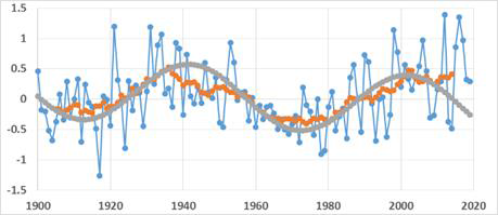
Tiny Towns Anomaly (blue), 11-yr Running, Centered Average (red),
and Sine Wave with Negative Linear Trend (0.29) deg C/100 Y (gray line) Pearson R=+0.9

The equation for the sine wave with a downward linear trend is shown in Equation 1.

Eqn. 1 𝑻𝒄𝒂𝒍𝒄=𝑺𝒊𝒏(𝟐∗𝑷𝒊𝟑𝟔𝟎∗(𝟔∗𝒀𝑬𝑨𝑹−𝟏𝟏𝟐𝟎𝟐))∗𝟎.𝟓−𝟎.𝟎𝟎𝟐𝟗∗𝒀𝑬𝑨𝑹+𝟓.𝟕𝟏

Where YEAR is the year in question, e.g. 1942. Tcalc is the calculated temperature anomaly in degrees C for the year in question.
The negative overall trend of minus 0.29 degrees C per century exists in spite of multiple, recent upward spikes in the data. These upward spikes are due to the severe drought of 2012, and large El Niño events in 1987, 1990-91, 1998, 2006, and 2015-16.

2.3 Data Validation

Five validation checks were performed. First, NOAA contiguous US data shows excellent agreement with the tiny towns’ annual anomalies. (Fig. 6) Second, the US Climate Reference Network, USCRN, also shows excellent agreement for the period 2005-2019 with Pearson R of +0.95. (Fig. 8). [12] Third, the Goodridge data for California counties from 1909-1994 also shows good agreement in simple linear trend and sinusoidal shape of the annual data for counties with very small populations (Fig. 3, lower line)

Figure 8
USCRN Anomalies (blue) and Tiny Towns Anomalies (red) 2005-2019, deg C

As mentioned, the tiny towns’ Pearson R coefficient is +0.9 for the 60-year sine wave model with negative linear trend when regressed against the 11-year running, centered average of the annual temperature anomalies. This is a very high correlation with very good significance at the 95 percent confidence level.

Fourth, this study was compared with the results of Loehle and Scafetta (2011) [13], who also found a 60 year cycle with a linear component over a similar period. The similarities with Loehle and Scafetta 2011 end there, however. Their proposed model includes a secondary cycle of 20 years. Also, they used full global data from HadCRUT3 for the period 1850 through 2010, and found a positive linear trend starting in 1942. The HadCRUT3 global data includes sites with various populations and record lengths, and therefore has warming due to human activities and data manipulations. Other differences include a cycle amplitude of approximately +0.16 degrees C, and minimum at year 1910. This study has a cycle amplitude of 0.5 degrees C, the minimum at year 1912, and a negative linear slope over the entire period 1900-2019. This study shows an overall cooling, but no warming. Fifth, Zeleňáková and Purcz (2015) [14] state that low-population areas have had no warming.

2.4 Factors in No Warming

One of the many factors that supports the conclusion of no warming from GHGs is the trivial, insignificant radiation of heat by atmospheric CO2. While it is true that CO2 is a luminous gas, there are four important parameters that govern its luminosity, or radiation of infra-red energy. Those parameters, or atmospheric conditions, disfavor any significant impact by CO2. The four parameters are 1) relatively low temperature, 2) very low CO2 concentration, 3) low pressure, and 4) extremely long mean beam length. Mean beam length is the average distance from radiating CO2 molecules to a heat-receiving surface. An excellent discussion of the parameters for CO2’s radiant properties as a luminous gas is given in Perry’s Chemical Engineers’ Handbook 7th Ed., Chapter 5. [15]

Another factor in no warming in remote, tiny towns is the following: only three data adjustments were needed in this study due to the data selection criteria. Four other adjustments contribute to the warming found in the NOAA, GISS, Hadley CRU, and BEST global temperature studies. The four adjustments that were not needed in this study are: UHI or Urban Heat Island effect, splicing together short records, infilling missing data, and averaging multiple locations within a grid. Those four adjustments appear to create a spurious warming that is then attributed to CO2.

At least eight other factors have an impact on warming trends. Those factors include 1) increased urban population density, 2) increased energy use per capita, and 3) increased local humidity. Also, 4) lower albedo from cleaner air as air pollution laws became effective, and 5) changes in cloud cover. Finally, 6) the severity and timing of droughts, 7) ENSO events, and 8) large volcanic eruptions. [9] Only the last five of those factors impact the remote, tiny towns. The first three of those factors do not affect the remote, tiny towns.

3 Conclusion and Implications

The instrumental temperature record of 82 remote, widespread, tiny towns in the US shows no warming from greenhouse gases over 120 years from 1900 through 2019. Instead, a slight cooling trend was found of minus 0.29 degrees C per century. The data showed a distinct cyclical pattern with period 60 years, amplitude 0.5 degrees C, and a minimum at year 1912. The goodness of fit was very high, as measured by the Pearson R coefficient of +0.9 when the cyclical fit with linear component was compared to an 11-year smoothed, running, and centered average of the annual data. The cooling trend is in good agreement with the results of Goodridge (1996), also Zeleňáková and Purcz (2015). However, this result is counter to the results from studies by BEST, GISS, NOAA for the globe, and NOAA for the contiguous US.

Since GHGs from human activity, primarily CO2, have no warming impact on locations in remote areas with tiny populations, there can be no GHG warming of medium and large cities either. Science cannot be arbitrary nor capricious. For GHGs to ignore tiny towns with very small populations requires the GHG-induced global warming hypothesis to be rejected. As Dr. Richard Feynman stated in his lectures at Cornell University in 1964 [16], “If it (the hypothesis) disagrees with experiment, it’s wrong. And that simple statement is the key to science. It doesn’t make any difference how beautiful your guess is, it doesn’t make any difference how smart you are, who made the guess, or what his name is. If it disagrees with experiment, it’s wrong. That’s all there is to it.” This study shows that the GHG warming hypothesis is invalid for 82 remote, tiny towns across the US over the past 120 years. There is thus no need for any policies or efforts to reduce human-caused GHGs. There is no need for international treaties, nor for a carbon tax to provide incentives to reduce CO2 emissions. Also, there is no need for CCUS systems for CO2 reduction, nor for a hydrogen-based economy. Finally, there is no need for bio-fuels nor nuclear power plants, when their economics can be justified only by a carbon-based subsidy. Any renewable energy or other low-carbon technologies must stand on their own merits without any subsidies from a carbon tax or similar support schemes.

4 Acknowledgements

This work was performed with no outside funding. Also, the author would like to acknowledge the tremendous impact of the late Richard P. “Straight-Line” Cline, P.E. in Chemical Engineering and P.E. in Civil Engineering. Dick shared with me his unending patience and deep knowledge of data analysis, and the conclusions that may be drawn from the data. His methods changed the world of oil refining for the great betterment of mankind.

5 Copyright Notice

Figure 3 is used under 17 U.S. Code §107, Limitations on Exclusive Rights: Fair Use. Figures 1 and 2 are used under 17 U.S. Code §105, US Government Works. All other Figures are Copyright © 2020 by Roger E. Sowell.

6 References

[1] NOAA National Center for Environmental Information – Climate At A Glance Global Time Series, Available at https://www.ncdc.noaa.gov/cag/global/time-series Accessed February 2, 2020.

[2] NOAA National Center for Environmental Information – Climate At A Glance National Time Series, Available at https://www.ncdc.noaa.gov/cag/national/time-series Accessed February 2, 2020.

[3] N. L. Bindoff, P.A. Stott, et. al., Detection and Attribution of Climate Change: from Global to Regional. In: Climate Change 2013: The Physical Science Basis. Contribution of Working Group I to the Fifth Assessment Report of the Intergovernmental Panel on Climate Change [Stocker, T.F., D. Qin, et. al. (eds.)]. Cambridge University Press, Cambridge, United Kingdom and New York, NY, USA, 2013

[4] United Nations Climate Change – The Paris Agreement, Available at https://unfccc.int/process-and-meetings/the-paris-agreement/the-paris-agreement, Accessed February 14, 2020

[5] Fifth Assessment Report of the IPCC – SUPPLEMENTARY MATERIAL Cambridge University Press, Cambridge, United Kingdom and New York, NY, USA, 2013, Figure AI.SM2.6.1

[6] J. D. Goodridge, Comments on “Regional Simulations of Greenhouse Warming including Natural Variability,” B Am Meterol Soc, 77, (1996), 1588-1599

[7] J. Hansen, R. Ruedy, M. Sato, K. Lo, GLOBAL SURFACE TEMPERATURE CHANGE, Rev Geoph 48 Issue 4 2010, 1-29

[8] C. Wickham, R. Rhode, R.A. Muller, J. Wurtele, J. Curry, et al., Influence of Urban Heating on the Global Temperature Land Average Using Rural Sites Identified from MODIS Classifications, Geoinfor Geostat: An Overview 2013, 1:2

[9] R. Sowell, Ten Causes of Global Warming – None is CO2, Available at https://sowellslawblog.blogspot.com/2017/03/ten-causes-of-global-warming-none-is-co2.html, Accessed February 2, 2020

[10] NOAA National Center for Environmental Information – Climate Data Online, Available at https://www.ncdc.noaa.gov/cdo-web/ Accessed February 2, 2020

[11] M. Menne, C. Williams, R. Vose, The US Historical Climatology Network monthly temperature data, version 2. B Am Meterol Soc 90 (2009), 993-1007

[12] NOAA National Center for Environmental Information – National Temperature Index, Available at https://www.ncdc.noaa.gov/temp-and-precip/national-temperature-index/, Accessed February 2, 2020

[13] C. Loehle and N. Scafetta, Climate Change Attribution Using Empirical Decomposition of Climatic Data, Open Atm Sci J, 5, (2011), 74-86

[14] M. Zeleňáková and P. Purcz, et. al., Climate Change In Urban Versus Rural Areas, Procedia Engineering, 119, (2015), 1171–1180

[15] R. H. Perry, D. W. Green, and J. O. Maloney, Perry’s Chemical Engineers’ Handbook, Seventh Ed., McGraw-Hill, New York, NY, 1997, 5-32 – 5-35.

[16] R. P. Feynman, Richard Feynman Messenger Lectures at Cornell The Character of Physical Law Part 7 Seeking New Laws, Available at https://youtu.be/-2NnquxdWFk at 17:20 min, Accessed on February 2, 2020

————————————- END of PAPER ———————————–